Optimal design of octet-truss lattices with FEniCS-adjoint

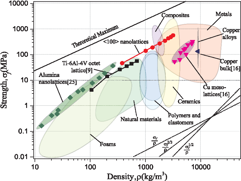
Modern technologies in additive manufacturing allow the design of structural components with a fine control on the small scale features. This opens up the design space to new materials with better mechanical properties. One such example is the octet-truss lattice, whose stiffness scales linearly with density ¹, instead of degrading as it happens with foams.

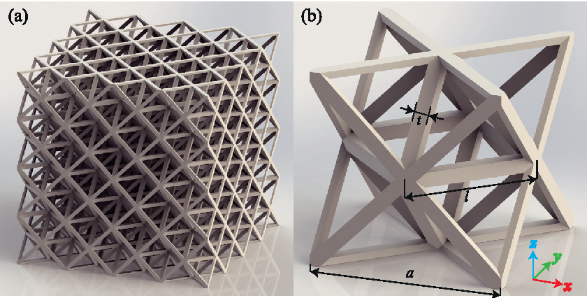
The design of octet-truss lattices requires accurate and efficient simulation methods. In this post, we will assume the lattice is comprised by stretch dominated slender members, behaving as structural trusses. We also assume periodicity of a characteristic unit cell throughout the lattice and a separation of scales, meaning the characteristic scale of the unit cell is much smaller than the dimensions of the overall structure. In this scenario, we can apply homogenization methods and obtain an equivalent continuum model of the structure, reducing the number of degrees of freedom necessary and saving computational time. This approach is therefore limited to structures where the unit cell is much smaller than the overall dimensions of the structure and to small deformations in the static linear elastic regime. There is abundant research going on to obtain better models for these lattices.

As such, our model is simply a linear elasticity equation whose elasticity tensor represents the octet-truss lattice in a continuum fashion.

$$ \begin{align} \nabla \cdot \mathbb{C}(\mathbf{a})[\nabla \mathbf{u}] + \mathbf{f} &= 0 &\text{in}~&\Omega \\ \mathbb{C}(\mathbf{a})[\nabla \mathbf{u}] \cdot \mathbf{n} &= \mathbf{t} &\text{in}~&\Gamma_N \end{align} $$

Our body load $\mathbf{f}$ is zero in our case and we will be using the equivalent weak form of the equations to be able to use the finite element method.

$$ \int_{D} \mathbb{C}(\mathbf{a})[\nabla \mathbf{u}]: \nabla \mathbf{v} ~dV + \int_{\Gamma_N} \mathbf{t} \cdot \mathbf{v} ~d\Gamma = 0 $$

The elasticity tensor $\mathbb{C}(\mathbf{a})$ captures the dependence on the design variables ². $$\mathbb{C}(\mathbf{a}) = \frac{E}{V_{\text{UC}}} \sum_{i=1}^{n_{struts}} a_i l_i \mathbf{n}_i \otimes \mathbf{n}_i \otimes\mathbf{n}_i \otimes\mathbf{n}_i$$ where $\mathbf{a}$ is the vector containing all trusses cross sections, $E$ is the Young modulus and $V_{\text{UC}}$ is the volume of the unit cell ($4 l^3 / \sqrt{2}$).

Optimization problem

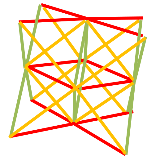
We are going to use three variables per unit cell, each one will define the cross section area of all the trusses in the XY, YZ and XZ planes, i.e. eight trusses per design variable per unit cell. In this figure, I am coloring the trusses per design variable. There are twelve per color, but only eight actually belong to the current unit cell. The remaining four belong to the next unit cell in the periodic lattice. We could have used more than three design variables per unit cell, but we leave it to three for sake of simplicity.

Our goal is to obtain a very stiff structure, therefore we minimize the compliance $$J(\mathbf{a}) = \int_{\Gamma_N} \mathbf{t} \cdot \mathbf{u}(\mathbf{a}) ~dV $$ subject to a volume constraint, otherwise the optimization would fill the entire domain with material, and we are interested in obtaining a lighter design.

$$ V(\mathbf{a}) = \int_{\Omega} 8 \sum_{i=1}^3 a_i l_i \rho ~dV - \hat{V} \leq 0 $$

Our structure is a simple cantilever beam with dimensions 30 by 10 by 10, clamped on the plane $x=0$ and with a load applied on $$\Gamma_N = \{ x=40 \cap 10 / 4 \leq y \leq 30 / 4 \cap 10 / 4 \leq z \leq 30 / 4 \}$$

Implementation

We use pyadjoint to calculate the gradients. pyadjoint keeps an interface to both FEniCS and Firedrake. Previous version of pyadjoint was called dolfin-adjoint.

First, import fenics and fenics_adjoint. fenics_adjoint overloads most of the fenics core operations to record them in a tape. This has the advantage of keeping the interface pretty similar while deriving the gradients automatically. Many more details on this library along with several examples can be found in their website. In this blog entry, I am following their topology optimization example.

from fenics import *
from fenics_adjoint import *

We next import the IPOPT python interface.

try:
    import pyipopt
except ImportError:
    print("""This example depends on IPOPT and pyipopt. \
  When compiling IPOPT, make sure to link against HSL, as it \
  is a necessity for practical problems.""")
    raise

Mesh geometry built with hexahedra. I am using hexahedra to have a geometric correspondence between the octet-truss unit cell and the mesh elements. It is worth mentioning that FEniCS support for hexahedra is currently limited (version 2019.1.0) to the built-in mesh constructors (UnitSquareMesh, UnitCubeMesh, RectangleMesh, BoxMesh, etc).

height = 10.0
width = 30.0
n_elem_side_y = 20
n_elem_side_x = 60
mesh = BoxMesh.create([Point(0, 0, 0), Point(width, height, height)], [n_elem_side_x, n_elem_side_y, n_elem_side_y], CellType.Type.hexahedron)

In the unit cell, the vectors that mark the trusses directions are simply oriented at 45 degrees with respect to each of the coordinates planes.

vectors = list(itertools.product([1.0/sqrt(2.0), -1.0/sqrt(2.0)],repeat=2))
vectors_np = np.array(vectors)
zeros_column = np.zeros((len(vectors),1))
n_xy = np.c_[vectors_np[:,[0]], vectors_np[:,[1]], zeros_column]
n_yz = np.c_[zeros_column, vectors_np[:,[0]], vectors_np[:,[1]]]
n_xz = np.c_[vectors_np[:,[0]], zeros_column, vectors_np[:,[1]]]

And we embed these vectors into UFL format to use them in our weak form.

vectors = list(itertools.product([1.0/sqrt(2.0), -1.0/sqrt(2.0)],repeat=2))
vectors_np = np.array(vectors)
zeros_column = np.zeros((len(vectors),1))
n_xy = np.c_[vectors_np[:,[0]], vectors_np[:,[1]], zeros_column]
n_yz = np.c_[zeros_column, vectors_np[:,[0]], vectors_np[:,[1]]]
n_xz = np.c_[vectors_np[:,[0]], zeros_column, vectors_np[:,[1]]]

The function space of the design variables is a piecewise discontinuous space with three components per element.

RHO = VectorFunctionSpace(mesh, "DG", 0)
A_list = Function(RHO, name='Control')
A_list.interpolate(Constant((0.1, 0.1, 0.1)))

The material properties of alumina are

E = 300e5 # N / cm^2
rho = 3.5 # Mg / m^3 or g / cm^3

The strain tensor and constitutive response.

def epsilon(u):
    return 0.5*(nabla_grad(u) + nabla_grad(u).T)

unit_cell_volume = length_truss**3 * 4.0 / np.sqrt(2.0)
from ufl import i, j, k, l
def sigma(r, A_list):
    # Factor 2 because this plane of struts is repeated twice in the unit cell
    Cijkl = [Constant(E) * 2.0 * length_truss * A_section / Constant(unit_cell_volume) *
            all_normals[index][row_index][i]*
            all_normals[index][row_index][j]*
            all_normals[index][row_index][k]*
            all_normals[index][row_index][l]
            for index, A_section in enumerate(split(A_list)) for row_index in range(4) ]
    C = as_tensor(sum(Cijkl), (i,j,k,l))
    return C[i,j,k,l]*epsilon(r)[k,l]

Boundary conditions. Clamped on one end and a load region on the other end.

class DirichletBoundary(SubDomain):
  def inside(self, x, on_boundary):
    return near(x[0], 0.0) and on_boundary

class NeumanBoundary(SubDomain):
  def inside(self, x, on_boundary):
    return near(x[0], width) and between(x[1], (height*1.0/4.0, height*3.0/4.0)) \
        and between(x[2], (height*1.0/4.0, height*3.0/4.0))

boundaries = MeshFunction('size_t', mesh, mesh.geometric_dimension() - 1)
NeumanBoundary().mark(boundaries, 2)
DirichletBoundary().mark(boundaries, 1)

ds = Measure('ds', domain=mesh, subdomain_data=boundaries)

We now proceed to solve the elasticity problem.

W = VectorFunctionSpace(mesh, "CG", 1)
v = TestFunction(W)
u = TrialFunction(W)

a = inner(epsilon(v)[i,j], sigma(u, A_list))*dx
traction = Constant((0.0, -10.0, 0.0))
L = inner(traction, v)*ds(2)

bc = DirichletBC(W, Constant((0.0, 0.0, 0.0)), boundaries, 1)

u_sol = Function(W)
solve(a==L, u_sol, bcs=[bc])

The compliance is our cost function, as we are interested in obtaining the stiffest possible structure.

J = assemble(inner(u_sol, traction)*ds(2))

For visualization purposes, we plot the design at each optimization iteration.

allctrls = File("output/allcontrols.pvd")
rho_viz = Function(RHO, name="ControlVisualisation")
def eval_derivative_cb(j, dj, vf):
    rho_viz.assign(vf)
    allctrls << rho_viz

Pyadjoint handles the optimization through the ReducedFunctional object to evaluate the compliance and its derivative throughout the optimization.

vf = Control(A_list)
Jhat = ReducedFunctional(J, vf, derivative_cb_post=eval_derivative_cb)

The constraints in our problems are bound constraints, as we do not want to have very thick or very small trusses and a mass constraint to limit the total amount of material to use. section area everywhere.

lb = 0.0001
ub = 0.005
V = assemble(Constant(rho)*dx(domain=mesh), annotate=False) / (n_elem_side_x*n_elem_side_y**2)
delta = 0.05  # Volume ratio for the trusses
trusses_per_plane = 4 * 3
mass_per_variable = length_truss * trusses_per_plane
mass_per_variable = length_truss * trusses_per_plane * rho
volume_constraint = UFLInequalityConstraint((V*delta - \
            mass_per_variable*(A_list[0] + A_list[1] + A_list[2]))*dx, vf)

We formulate the optimization problem

problem = MinimizationProblem(Jhat, bounds=(lb, ub), constraints=volume_constraint)
parameters = {'maximum_iterations': 100}

and solve it

solver = IPOPTSolver(problem, parameters=parameters)
rho_opt = solver.solve()

The final result is plotted in ParaView with a VTK script found here (it's a bit slow since it is looping in python).

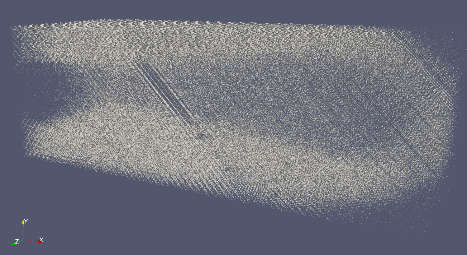
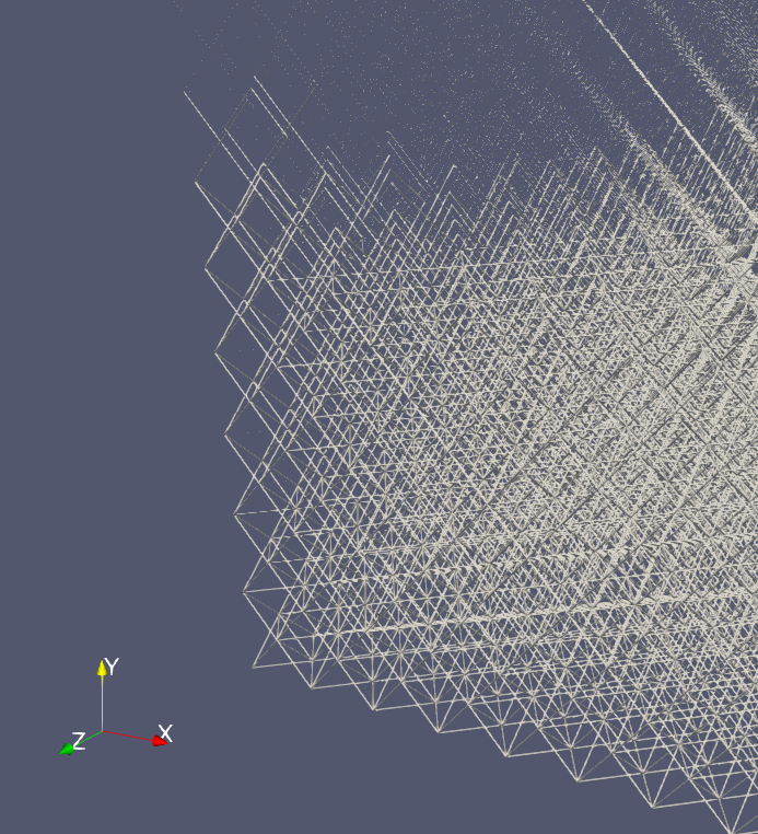
You will need to zoom in to see the lattice detail, I decided to include it just to show the overall beam structure with more material at the top and bottom to increase the moment of inertia.

Here I am showing in detail the lattice at the bottom right corner, where the anisotropy in the struss areas is more visible.

For visualization purposes, here is a three dimensional plot of a similar problem with a much coarser mesh. It is a heavy file that takes few seconds to load.

The code to run this optimization and the visualization can be found here.