Topology optimization of fluid-based problems with open source code

This is my attempt to show how to solve a fluid-based topology optimization problem using open source code. Instead of solving the trivial case of power dissipation minimization, I will tackle a more interesting example: A fixed-geometry fluid diode that minimizes the pressure drop of the flow in one direction and maximizes it in the opposite direction. In other words, it is easier for the fluid to flow in one direction and more difficult in the other direction.

This is the idea behind the original Tesla valve, created by Nikola Tesla more than a century ago. The topology optimization community has emulated this design with an automated framework, opening up the possibility of extending the idea to more complex geometries and three-dimensions. This is what Lin et al¹ have done and I attempt to reproduce their results here. Their article is available on ResearchGate.

We model the flow with the nondimensional Navier-Stokes equation

$$ \begin{align} \mathbf{u}\cdot \nabla \mathbf{u} + \alpha(\rho) \mathbf{u}-\frac{1}{Re} \nabla^{2} \mathbf{u}+\nabla p & =f & & \text { in } \Omega \\ \operatorname{div}(\mathbf{u}) &=0 & & \text { in } \Omega \\ \mathbf{u} &=\mathbf{u}_{\text{in}} & & \text { on } \Gamma_{\text{in}} \\ \frac{1}{Re} \nabla \mathbf{u} \cdot \mathbf{n}-p \mathbf{n}&=0 && \text { on } \Gamma_{\text {out}}\\ \mathbf{u} &=0 & & \text { on } \Gamma_{\text{wall}}\,, \end{align} $$

where $Re$ is the Reynolds number, $\mathbf{u}$ and $p$ are the fluid velocity and pressure. The vector normal to the boundary is denoted with $\mathbf{n}$. The Brinkmann term $\alpha(\rho)\mathbf{u}$ models the solid domain as a nearly impermeable material. For values of the volume fraction $\rho = 0$, i.e. the solid domain, the Brinkmann term dominates the Navier-Stokes equation which results in a negligible fluid velocity. On the other hand, for $\rho=1$, the flow velocity is not affected. To penalize values of $\rho$ between 0 and 1 that do not have physical meaning, we use the RAMP function³.

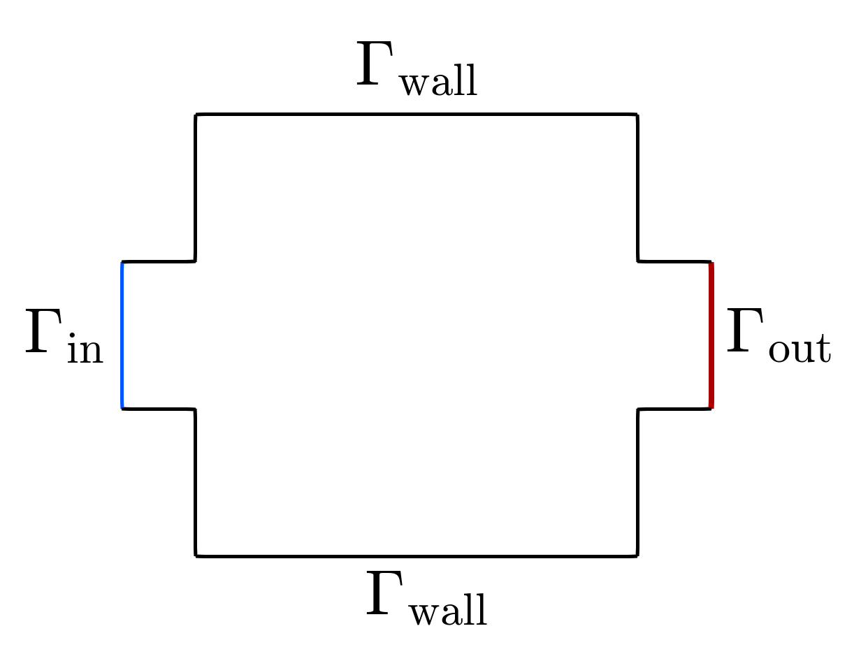
In the figure below, the forward fluid flows from $\Gamma_{\text{in}}$, where a sinusoidal profile on the velocity $\mathbf{u}_{\text{in}}$ is imposed, to $\Gamma_{\text{out}}$, where there is zero traction. I should have used a parabolic profile to have a more realistic velocity profile. This is left for future implementation. The reverse fluid flows in the opposite direction. Therefore, in the above equations, the boundary conditions on $\Gamma_{\text{in}}$ and $\Gamma_{\text{out}}$ are simply switched.

The performance of the liquid diodes is the diodicity, i.e., the ratio of the pressure drop of the reverse flow to the pressure drop in the forward flow. Since the goal is to impede reverse flow and facilitate forward flow, we maximize the diodicity. As in Lin et al¹, we use power dissipation instead of pressure drop because, in topology optimization, it is better to use cost functions that are volume/area integrals rather than facet integrals. Therefore, we calculate the power dissipation as follows

$$ \phi(\rho, \mathbf{u}(\rho)) =\int_{\Omega} \alpha(\rho) \mathbf{u} \cdot \mathbf{u}~d\Omega+\frac{1}{Re} \int_{\Omega} \nabla \mathbf{u}: \nabla \mathbf{u}~d\Omega $$

and the diodicity as

$$ Di = \frac{\phi(\rho, \mathbf{u}_r)}{\phi(\rho, \mathbf{u}_f)} $$

As noted by Lin et al¹, simply using the diodicy as the cost function leads to designs with pockets of intermediate material. To eliminate them, Lin et al¹ adds a penalty term to the cost function to penalize the flow through the solid and intermediate phases in the reverse direction.

$$ F_* = \int_{\Omega} \alpha(\rho) \mathbf{u}_r \cdot \mathbf{u}_r~d\Omega $$

Lastly, we use the filter method² to maintain a minimum length scale and avoid very thin channels in the optimized design. Unlike in Lin et al¹, here we do not use a projection method, which would add complexity in the convergence of the optimization algorithm. The downside is that our design boundaries are not as clearly defined, but still good enough.

Putting it all together, our optimization problem statement is

$$ \begin{align} \underset{\rho}{\text{min}}~\frac{1}{Di} + \cdot F_* \\ \text{s.t.: }\mathbf{u}_f \cdot \nabla \mathbf{u}_f + \alpha(\hat\rho) \mathbf{u}_f -\frac{1}{Re} \nabla^{2} \mathbf{u}_f +\nabla p_f & =0 & & \text { in } \Omega \\ \operatorname{div}(\mathbf{u}_f ) &=0 & & \text { in } \Omega \\ \mathbf{u}_f &=\mathbf{u}_{\text{in}_f } & & \text { on } \Gamma_{\text{in}} \\ \frac{1}{Re} \nabla \mathbf{u}_f \cdot \mathbf{n}-p_f \mathbf{n}&=0 && \text { on } \Gamma_{\text {out}}\\ \mathbf{u}_r &=0 & & \text { on } \Gamma_{\text{wall}}\\ \mathbf{u}_r \cdot \nabla \mathbf{u}_r + \alpha(\hat\rho) \mathbf{u}_r -\frac{1}{Re} \nabla^{2} \mathbf{u}_r +\nabla p_r & =0 & & \text { in } \Omega \\ \operatorname{div}(\mathbf{u}_r ) &=0 & & \text { in } \Omega \\ \mathbf{u}_r &=\mathbf{u}_{\text{in}_r } & & \text { on } \Gamma_{\text{out}} \\ \frac{1}{Re} \nabla \mathbf{u}_r \cdot \mathbf{n}-p_r \mathbf{n}&=0 && \text { on } \Gamma_{\text {in}}\\ \mathbf{u}_r &=0 & & \text { on } \Gamma_{\text{wall}}\\ \kappa \nabla^2 \hat\rho + \hat\rho &= \rho& & \text { in } \Omega \\ 0 \leq \rho &\leq 1 \\ \int_{\Omega} \hat\rho~dV &\leq V_{\text{max}}\int_{\Omega} dV \,. \end{align} $$

The PDE filter equation with a filter parameter $\kappa$ solves for the filtered volume fraction $\hat\rho$, which is fed to the Navier-Stokes equations through the Brinkman term $\alpha(\hat\rho)\mathbf{u}$. The volume constraint is added to prevent undesirable local minima and it is not necessarily always active. Here we use $V_{\text{max}} = 0.7$.

We start importing the necessary modules and declaring the variables for the mesh markers used in diode.geo.

import argparse
import firedrake as fd
from firedrake import inner, dot, grad, div, dx, ds, pi
import firedrake_adjoint as fda
from pyadjoint.placeholder import Placeholder
from pyMMAopt import MMASolver, ReducedInequality
from filter import pde_filter
from penalization import ramp

DOMAIN = 5
INMOUTH = 6
OUTMOUTH = 7
INLET_WIDTH = 1.0
Y_INLET = 0.5

The script has a command-line argument to set up the directory to save the results.

def navier_stokes_flow():

    parser = argparse.ArgumentParser(description="")
    parser.add_argument(
        "--output-dir",
        dest="output_dir",
        type=str,
        action="store",
        default="./",
        help="Directory where to save the result",
    )

    opts = parser.parse_args()
    output_dir = opts.output_dir

The problem size is small enough to use a direct solver.

    solver_parameters_direct = {
        "snes_atol": 1e-7,
        "mat_type": "aij",
        "pc_type": "lu",
        "pc_factor_mat_solver_type": "mumps",
        "mat_mumps_icntl_14": 200,
        "mat_mumps_icntl_24": 1,
    }

Both flow problems differ only in their inlet and outlet boundary conditions.

    boundary_conditions_forward = {
        "INLET": 1,
        "OUTLET": 2,
        "WALLS": 3,
        "ZERO_NORMAL": 4,
    }
    boundary_conditions_reverse = {
        "OUTLET": 1,
        "INLET": 2,
        "WALLS": 3,
        "ZERO_NORMAL": 4,
    }

Load the mesh and create the function spaces for the control and the flow variables: velocity and pressure.

    mesh = fd.Mesh("./diode.msh")

    RHO = fd.FunctionSpace(mesh, "DG", 0)
    V = fd.VectorFunctionSpace(mesh, "CG", 2)
    Q = fd.FunctionSpace(mesh, "CG", 1)
    W = V * Q

Next, some parameters that define the problem. The Reynolds number, which must be high enough to obtain interesting designs and the Darcy number, which must be low enough to make the solid material behave like a non-porous material. Darcy numbers that are too low can hinder convergence. For this reason, we will continue to decrease it during the optimization. We use the Placeholder class in pyadjoint to facilitate this operation. More details on how to use this class are in this pyadjoint example. The ramp_p constant measures the degree of the RAMP penalty scheme.

    Re = fd.Constant(300.0)
    Da = fd.Constant(1e-4)
    Placeholder(Da)
    ramp_p = fd.Constant(10.0)

Initialize the control variable and filter it using a Two-Point Flux Approximation scheme. Using this discretization method for the PDE filter is not a problem here because the mesh is mostly composed of equilateral triangles. In the future, I plan to switch back to the traditional Lagrange finite elements.

    with fda.stop_annotating():
        rho = fd.interpolate(fd.Constant(0.5), RHO)

    rhof = pde_filter(
        RHO,
        rho,
        filter_radius=fd.Constant(1e-4),
        solver_parameters=solver_parameters_direct,
    )
    rhof_control = fda.Control(rhof)

The inlet flow is fully developed and follows a sinusoidal profile with half a period.

    _, y = fd.SpatialCoordinate(W.ufl_domain())

    def inflow(u_inflow):
        return fd.as_vector(
            [
                -u_inflow * fd.sin(((y - (Y_INLET)) * pi) / INLET_WIDTH),
                0.0,
            ]
        )

Now we can create and solve the forward problem,

    u_inflow = 1.0
    inflow_forward = inflow(u_inflow)
    up_forward = flow_problem(
        W,
        rhof,
        Re,
        Da,
        ramp_p,
        boundary_conditions_forward,
        inflow_forward,
        ramp,
        solver_parameters=solver_parameters_direct,
    )
    u_f, _ = fd.split(up_forward)

and the reverse problem, more details on flow_problem routine are below

    inflow_reverse = inflow(-u_inflow)
    up_reverse = flow_problem(
        W,
        rhof,
        Re,
        Da,
        ramp_p,
        boundary_conditions_reverse,
        inflow_reverse,
        ramp,
        solver_parameters=solver_parameters_direct,
    )
    u_r, _ = fd.split(up_reverse)

Some files and auxiliary variables to plot the evolution of the design and the velocity fields.

    plot_file = f"{output_dir}/design.pvd"
    controls_f = fd.File(plot_file)
    vel_pvd = fd.File("velocity.pvd")
    up_control_f = fda.Control(up_forward)
    up_control_r = fda.Control(up_reverse)
    rho_viz_f = fd.Function(RHO, name="rho")

    def deriv_cb(j, dj, rho):
        with fda.stop_annotating():
            rho_viz_f.assign(rhof_control.tape_value())
            u_plot, p_plot = up_control_f.tape_value().split()
            u_plot.rename("Velocity")
            p_plot.rename("Pressure")
            u_plot_r, p_plot_r = up_control_r.tape_value().split()
            u_plot_r.rename("Velocity reverse")
            p_plot_r.rename("Pressure reverse")
            vel_pvd.write(u_plot, p_plot, u_plot_r, p_plot_r)
            controls_f.write(rho_viz_f)

Next, we calculate the power dissipation for both the forward and reverse flows. We combine these two quantities to calculate the diodicity $Di$ and add a penalization term to remove residual regions with intermediate material as in Lin et al¹.

    G = power_dissipation(u_f, rhof, Re, Da, penalization=ramp, ramp_p=ramp_p)
    G_reverse = power_dissipation(u_r, rhof, Re, Da, penalization=ramp, ramp_p=ramp_p)
    Wf = 1.0
    Diodicity = fda.AdjFloat(1.0) / (G_reverse / G) + fd.assemble(
        Wf
        * alpha(rhof, Da, penalization=ramp, ramp_p=ramp_p)
        * inner(u_r, u_r)
        * dx(DOMAIN)
    )
    c = fda.Control(rho)
    Ghat = fda.ReducedFunctional(Diodicity, c, derivative_cb_post=deriv_cb)

We also create the volume constraint

    Vol = fd.assemble((rhof) * dx(DOMAIN))
    Vhat = fda.ReducedFunctional(Vol, c)
    Vcontrol = fda.Control(Vol)
    with fda.stop_annotating():
        Vlimit = 0.7 * fd.assemble(fd.Constant(1.0) * dx(DOMAIN, domain=mesh))

and finally, we initiate the continuation loop to iterate over the Darcy numbers that range from large to small values to avoid undesirable local minima.

Within the continuation loop, we create the MinimizationProblem and solve the optimization problem for a maximum number of iterations max_iter for each stage of the continuation loop. The optimized design rho_opt serves as the initial design for the next iteration in the continuation strategy.

    Da_arr = [1e-3, 5e-4, 2e-4]
    max_iter_arr = [50, 50, 1000]
    for Da_val, max_iter in zip(Da_arr, max_iter_arr):
        Da.assign(Da_val)

        lb = 0.0
        ub = 1.0

        problem = fda.MinimizationProblem(
            Ghat,
            bounds=(lb, ub),
            constraints=[
                ReducedInequality(Vhat, Vlimit, Vcontrol),
            ],
        )

        parameters_mma = {
            "move": 0.01,
            "maximum_iterations": max_iter,
            "m": 1,
            "norm": "L2",
            "gcmma": False,
        }
        solver = MMASolver(problem, parameters=parameters_mma)

        results = solver.solve()
        rho_opt = results["control"]
        with fda.stop_annotating():
            rho.assign(rho_opt)

What follows are the routines that define the physics in the optimization problem.

We first formulate the Navier-Stokes equation with the Brinkmann term, add the Galerkin Least-Squares stabilization, impose the boundary conditions and solve for the velocity and pressure. The routine accepts the boundary conditions as argument so that we can reuse it for both flows.

def flow_problem(
    W,
    rhof,
    Re,
    Da,
    ramp_p,
    boundary_conditions,
    inflow1,
    penalization,
    solver_parameters=None,
):

    v, q = fd.TestFunctions(W)

    up1 = fd.Function(W)
    u1, p1 = fd.split(up1)
    F1 = (
        1.0 / Re * inner(grad(u1), grad(v)) * dx
        + inner(dot(grad(u1), u1), v) * dx
        - p1 * div(v) * dx
        + div(u1) * q * dx
        + alpha(rhof, Da, penalization=penalization, ramp_p=ramp_p)
        * inner(u1, v)
        * dx(DOMAIN)
    )
    F1 = F1 + GLS(u1, v, p1, q, rhof, Da, Re, penalization=penalization, ramp_p=ramp_p)

    # Dirichelt boundary conditions
    noslip = fd.Constant((0.0, 0.0))
    bcs1_1 = fd.DirichletBC(W.sub(0), noslip, boundary_conditions["WALLS"])
    bcs1_2 = fd.DirichletBC(W.sub(0), inflow1, boundary_conditions["INLET"])
    bcs1_3 = fd.DirichletBC(
        W.sub(0).sub(1), fd.Constant(0.0), boundary_conditions["ZERO_NORMAL"]
    )
    bcs1 = [bcs1_1, bcs1_2, bcs1_3]

    problem = fd.NonlinearVariationalProblem(F1, up1, bcs=bcs1)
    solver = fd.NonlinearVariationalSolver(problem, solver_parameters=solver_parameters)
    solver.solve()

    return up1

Brinkmann parameter with the RAMP scheme to penalize intermediate volume fraction values.

def alpha(rho, Da, penalization=ramp, ramp_p=10.0):
    return (
        fd.Constant(1.0) / Da * penalization(rho, ramp_p=ramp_p, val_0=1.0, val_1=0.0)
    )

Galerkin Least-Square stabilization to manage the $P^1$-$P^1$ velocity-pressure discretization and higher Reynolds numbers.

def GLS(u, v, p, q, rhof, Da, Re, penalization=ramp, ramp_p=10.0):
    """
    Outside of design domain DOMAIN:
    GLS = tau_gls * inner(R_U, theta_u) * dx(OUTSIDE)
    Inside of design domain
    GLS = tau_gls_alpha * inner(R_U + R_U_alpha, theta_U + theta_U_alpha) * dx(DOMAIN)
    """
    R_U = dot(u, grad(u)) - 1.0 / Re * div(grad(u)) + grad(p)
    R_U_alpha = alpha(rhof, Da, penalization=penalization, ramp_p=ramp_p) * u
    theta_U = dot(u, grad(v)) - 1.0 / Re * div(grad(v)) + grad(q)
    theta_U_alpha = alpha(rhof, Da, penalization=penalization, ramp_p=ramp_p) * v
    mesh = rhof.function_space().ufl_domain()
    h = fd.CellDiameter(mesh)

    beta_gls = 0.5
    # beta_gls = 30.0
    tau_gls = fd.Constant(beta_gls) * (
        (4.0 * dot(u, u) / h ** 2) + 9.0 * (4.0 / (Re * h ** 2)) ** 2
    ) ** (-0.5)
    tau_gls_alpha = fd.Constant(beta_gls) * (
        (4.0 * dot(u, u) / h ** 2)
        + 9.0 * (4.0 / (Re * h ** 2)) ** 2
        + (alpha(rhof, Da, penalization=penalization, ramp_p=ramp_p)) ** 2
    ) ** (-0.5)

    return tau_gls * inner(R_U, theta_U) * (
        dx(INMOUTH) + dx(OUTMOUTH)
    ) + tau_gls_alpha * inner(R_U + R_U_alpha, theta_U + theta_U_alpha) * dx(DOMAIN)

Power dissipation routine used as cost function.

def power_dissipation(u, rhof, Re, Da, penalization, ramp_p):
    return fd.assemble(
        1.0 / Re * inner(grad(u), grad(u)) * dx
        + alpha(rhof, Da, penalization=penalization, ramp_p=ramp_p)
        * inner(u, u)
        * dx(DOMAIN)
    )

and finally, launch the script.

if __name__ == "__main__":
    navier_stokes_flow()

The optimized geometry below maximizes the diodicity of the system. The forward flow is fairly straight whereas the reverse flow has to sort out several sharp turns that increase the power necessary to pump fluid from right to left.

Evolution of the geometry throughout the optimization and the forward flow field.

Evolution of the geometry throughout the optimization and the reverse flow field.

From here, one could extend this script to design three-dimensional diodes. The first step is to replace the solver options for the Navier-Stokes equation. The direct solver used here does not scale for 3D problems and iterative solvers are needed. Such solvers exist in the literature for solving 3D fluid problems, but the inclusion of the Brinkmann term in our equations does not ensure that they will work for our problem. Indeed, only a SIMPLE-like solver with limited Reynolds number and for a particular geometry has worked for me.⁴

My understanding from interacting with the topology optimization community is that a geometric multigrid solver with the Galerkin-projection approach for the coarser matrices works well. Firedrake does have a geometric multigrid solver, but their implementation does not use the Galerkin-projection approach to build the coarser matrices. Instead, they simply rediscretize the equations in the coarser grid and assemble the matrix. This approach is fine for problems with uniform fields, but not for topology optimization, where the volume fraction field is a non-uniform field. Fortunately, PETSc, the linear algebra backend that Firedrake uses, does have an implementation of the Galerkin-projection. To use it, one would simply need to write the interpolation and restriction operators from Firedrake.

I hope you have found this post useful. You can find the code in this Github repository. If you have any questions, post an issue there and I will try to help.